

How To Change Tip Labels Of A Tree In R
ggtree Utilities
Facet Utilities
facet_widths
Adjusting relative widths of facet panels is a mutual requirement, especially for using geom_facet() to visualize a tree with associated information. Withal, this is not supported by the ggplot2 packet. To accost this outcome, ggtree provides the facet_widths() role and information technology works with both ggtree and ggplot objects.
library ( ggplot2 ) library ( ggtree ) library ( reshape2 ) set.seed ( 123 ) tree <- rtree ( 30 ) p <- ggtree ( tree, branch.length = "none" ) + geom_tiplab ( ) + theme (legend.position= 'none' ) a <- runif ( xxx, 0,one ) b <- 1 - a df <- information.frame ( tree $ tip.label, a, b ) df <- cook ( df, id = "tree.tip.label" ) p2 <- p + geom_facet (panel = 'bar', data = df, geom = geom_bar, mapping = aes (x = value, make full = every bit.factor ( variable ) ), orientation = 'y', width = 0.8, stat= 'identity' ) + xlim_tree ( 9 ) facet_widths ( p2, widths = c ( 1, two ) ) It too supports using a proper name vector to set the widths of specific panels. The following code will display an identical effigy to Figure 12.1A.
The facet_widths() role as well works with other ggplot objects as demonstrated in Figure 12.1B.

Effigy 12.1: Arrange relative widths of ggplot facets. The facet_widths() function works with ggtree (A) as well as ggplot (B).
facet_labeller
The facet_labeller() part was designed to relabel selected panels (Figure 12.2), and it currently merely works with ggtree objects (i.e., geom_facet() outputs). A more versatile version that works with both ggtree and ggplot objects is implemented in the ggfun package (i.e., the facet_set() office).
If y'all want to combine facet_widths() with facet_labeller(), you need to call facet_labeller() to relabel the panels before using facet_widths() to gear up the relative widths of each console. Otherwise, it won't work since the output of facet_widths() is redrawn from grid object.

FIGURE 12.2: Rename facet labels. Rename multiple labels simultaneously (A) or only for a specific i (B) are all supported. facet_labeller() tin combine with facet_widths() to rename facet label and then adjust relative widths (B).
Geometric Layers
Subsetting is not supported in layers defined in ggplot2, while it is quite useful in phylogenetic annotation since information technology allows united states to annotate at specific node(s) (eastward.m., only label bootstrap values that are larger than 75).
In ggtree, we provide several modified versions of layers defined in ggplot2 to support the subset aesthetic mapping, including:
-
geom_segment2() -
geom_point2() -
geom_text2() -
geom_label2()
These layers works with both ggtree and ggplot2 (Figure 12.3).

FIGURE 12.iii: Geometric layers that support subsetting. These layers work with ggplot2 (A) and ggtree (B).
Layout Utilities
In session 4.ii, we innovate several layouts supported by ggtree. The ggtree package also provides several layout functions that tin transform from 1 to another. Note that not all layouts are supported (see Tabular array 12.1 and Figure 12.4).
| Layout | Clarification |
|---|---|
| layout_circular | transform rectangular layout to round layout |
| layout_dendrogram | transform rectangular layout to dendrogram layout |
| layout_fan | transform rectangular/circular layout to fan layout |
| layout_rectangular | transform round/fan layout to rectangular layout |
| layout_inward_circular | transform rectangular/circular layout to inward_circular layout |

FIGURE 12.four: Layout functions for transforming amid different layouts. Default rectangular layout (A); transform rectangular to dendrogram layout (B); transform circular to rectangular layout (C); transform rectangular to circular layout (D); transform rectangular to fan layout (E); transform rectangular to inward round layout (F).
Scale Utilities
The ggtree parcel provides several calibration functions to dispense the ten-centrality, including the scale_x_range() documented in session v.2.4, xlim_tree(), xlim_expand(), ggexpand(), hexpand() and vexpand().
Expand x limit for a specific facet panel
Sometimes we demand to set xlim for a specific facet panel (eastward.g., allocate more space for long tip labels at Tree panel). Notwithstanding, the ggplot2::xlim() role applies to all the panels. The ggtree provides xlim_expand() to adjust xlim for user-specific facet panel. It accepts two parameters, xlim, and panel, and tin can adapt all private panels as demonstrated in Figure 12.5A. If you just want to adjust xlim of the Tree panel, yous tin use xlim_tree() every bit a shortcut.
The xlim_expand() function also works with ggplot2::facet_grid(). Every bit demonstrated in Figure 12.5B, just the xlim of virginica panel was adjusted by xlim_expand().

FIGURE 12.five: Setting xlim for user-specific facet panels. Using xlim_tree() to set the Tree panel of the ggtree output (A) and xlim_expand() to set the Dot console of the ggtree output (A) and the Virginica panel of the ggplot output (B).
Expand plot limit by the ratio of plot range
The ggplot2 package cannot automatically adjust plot limits and it is very common that long text was truncated. Users need to arrange x (y) limits manually via the xlim() (ylim()) command (see likewise FAQ: Tip characterization truncated).
The xlim() (ylim()) is a good solution to this outcome. Notwithstanding, we tin can make it more elementary, by expanding the plot console past a ratio of the axis range without knowing what the exact value is.
We provide hexpand() function to expand x limit past specifying a fraction of the x range and it works for both directions (management=i for right-manus side and direction=-1 for left-hand side) (Figure 12.6). Some other version of vexpand() works with like behavior for y-axis and the ggexpand() office works for both 10- and y-axis (Figure 11.two).
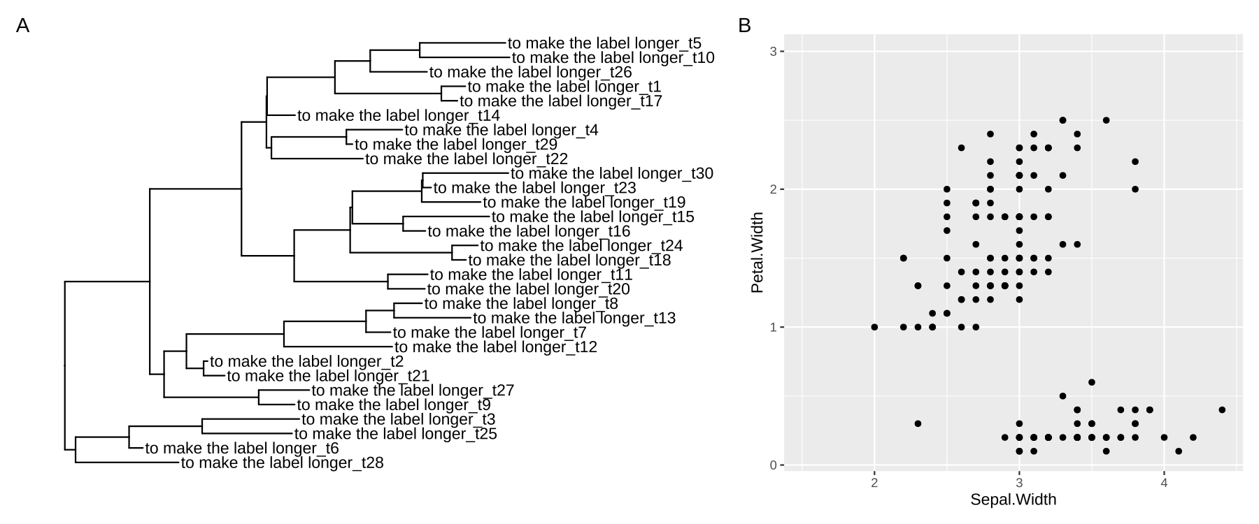
Figure 12.6: Expanding plot limits by a fraction of the x or y range. Aggrandize x limit at right-hand side by default (A), and aggrandize x limit for left-hand side when direction = -1 and expand y limit at the upper side (B).
Tree data utilities
Filter tree information
The ggtree package defined several geom layers that support subsetting tree data. However, many other geom layers that didn't provide this feature, are defined in ggplot2 and its extensions. To allow filtering tree data with these layers, ggtree provides an accompanying office, td_filter() that returns a office that works like to dplyr::filter() and tin be passed to the data parameter in geom layers to filter ggtree plot data as demonstrated in Effigy 12.seven.

Effigy 12.7: Filtering ggtree plot information in geom layers. Only selected tips (offspring of the node indicated by the blue circle point) were labeled.
Flatten list-column tree data
The ggtree plot information is a tidy data frame where each row represents a unique node. If multiple values are associated with a node, the data can be stored as nested information (i.e., in a list-column).
set.seed ( 1997 ) tr <- rtree ( 5 ) d <- data.frame (id= rep ( tr $ tip.label,ii ), value= abs ( rnorm ( x, 6, 2 ) ), group= c ( rep ( "A", five ),rep ( "B",5 ) ) ) crave ( tidyr ) d2 <- nest ( d, value = value, group= group ) ## d2 is a nested data d2 ## # A tibble: v × iii ## id value group ## <chr> <list> <list> ## 1 t2 <tibble [2 × one]> <tibble [2 × 1]> ## 2 t1 <tibble [2 × 1]> <tibble [2 × 1]> ## 3 t5 <tibble [2 × 1]> <tibble [2 × 1]> ## 4 t4 <tibble [2 × one]> <tibble [2 × 1]> ## five t3 <tibble [2 × 1]> <tibble [2 × ane]> Nested data is supported by the operator, %<+%, and can be mapped to the tree structure. If a geom layer can't directly back up visualizing nested data, nosotros demand to flatten the information earlier applying the geom layer to brandish it. The ggtree parcel provides a function, td_unnest(), which returns a function that works like to tidyr::unnest() and can be used to flatten ggtree plot information equally demonstrated in Figure 12.8A.
All tree data utilities provide a .f parameter to pass a function to pre-operate the information. This creates the possibility to combine different tree data utilities as demonstrated in Figure 12.8B.
p <- ggtree ( tr ) %<+% d2 p2 <- p + geom_point ( aes ( x, y, size= value, colour= group ), information = td_unnest ( c ( value, group ) ), alpha= .4 ) + scale_size (range= c ( 3,x ), limits= c ( 3, 10 ) ) p3 <- p + geom_point ( aes ( x, y, size= value, colour= group ), data = td_unnest ( c ( value, group ), .f = td_filter ( isTip & node == 4 ) ), alpha= .4 ) + scale_size (range= c ( 3,10 ), limits= c ( three, 10 ) ) plot_list ( p2, p3, tag_levels = 'A' ) 
Effigy 12.8: Flattening ggtree plot data. List-columns tin be flattened by td_unnest() and two circle points were displayed on each tip simultaneously (A). Different tree data utilities tin can be combined to piece of work together, due east.g., filter data by td_filter(), and and then flatten information technology past td_unnest()) (B).
Tree Utilities
Extract tip guild
To create blended plots, users demand to re-order their data manually earlier creating tree-associated graphs. The gild of their information should be consequent with the tip order presented in the ggtree() plot. For this purpose, nosotros provide the get_taxa_name() function to extract an ordered vector of tips based on the tree construction plotted by ggtree().
The get_taxa_name() part volition return a vector of ordered tip labels co-ordinate to the tree construction displayed in Figure 12.nine.
## [one] "t9" "t8" "t3" "t2" "t7" "t10" "t1" "t5" ## [ix] "t6" "t4" If users specify a node, the get_taxa_name() will extract the tip order of the selected clade (i.e., highlighted region in Figure 12.9).
## [1] "t5" "t6" "t4" Padding taxa labels
The label_pad() function adds padding characters (default is ·) to taxa labels.
## label newlabel ## 1 t1 ··················t1 ## 2 long cord for exam long cord for test ## iii t2 ··················t2 ## four t4 ··················t4 ## five t3 ··················t3 ## newlabel2 ## i t1 ## ii long string for exam ## 3 t2 ## 4 t4 ## 5 t3 This feature is useful if we desire to align tip labels to the stop as demonstrated in Figure 12.x. Note that in this case, monospace font should be used to ensure the lengths of the labels displayed in the plot are the same.
p <- ggtree ( tree ) %<+% d + xlim ( NA, 5 ) p1 <- p + geom_tiplab ( aes (label= newlabel ), align= TRUE, family unit= 'mono', linetype = "dotted", linesize = .7 ) p2 <- p + geom_tiplab ( aes (label= newlabel2 ), marshal= Truthful, family= 'mono', linetype = Cypher, offset= - .5 ) + xlim ( NA, five ) plot_list ( p1, p2, ncol= two, tag_levels = "A" ) 
Figure 12.ten: Align tip characterization to the end. With a dotted line (A) and without a dotted line (B).
Interactive ggtree Annotation
The ggtree package supports interactive tree annotation or manipulation by implementing an identify() method. Users can click on a node to highlight a clade, to characterization or rotate it, etc. Users can also utilise the plotly package to convert a ggtree object to a plotly object to speedily create an interactive phylogenetic tree.
Effigy 12.11: Interactive phylogenetic tree using place() method. Highlighting, labelling and rotating clades are all supported.
Video of using place() to interactively manipulate a phylogenetic tree can exist found on Youtube and Youku:
- Highlighting clades: Youtube and Youku.
- Labelling clades: Youtube and Youku.
- Rotating clades: Youtube and Youku.

How To Change Tip Labels Of A Tree In R,
Source: https://yulab-smu.top/treedata-book/chapter12.html
Posted by: smithfelich1959.blogspot.com
0 Response to "How To Change Tip Labels Of A Tree In R"
Post a Comment